
Using XLOOKUP in Excel
eCatholic ChMS offers many different reports. If you're hoping to generate a report that we don't currently offer, you may be able to generate reports that are readily available and then use an XLOOKUP function in Excel to pull in any additional data you need.
For instance, perhaps you'd like to see member information, but you'd like to include whether or not their family is registered at the parish. This is the example we will be diving into today, but the same general instructions can be applied to other downloads and datapoints.
IN THIS ARTICLE:
XLOOKUP Video Tutorial
Please click HERE to watch a step-by-step video tutorial of how to use the XLOOKUP function in Excel. This tutorial walks you through the example we described above—generating member information and adding a field to see whether or not their family is registered.
XLOOKUP Written Instructions
This is a long article that can feel overwhelming. Take it step-by-step and go as slow as you'd like. You may not even want to read the instructions. If not, simply watch the video above and you may find that that's enough to get you what you need. If you do prefer to read the instructions then keep on reading 😁
Step 1: Generating the Downloads
Important Note: In order to use the XLOOKUP function, you will need to have one unique field that is found in both downloads. This will more than likely be the Family ID field as it is the most unique datapoint that is tied to each family.
If Family ID is not available in both downloads, you can use Family Name or another field. Regardless of which field you choose you will just want to ensure that the field is unique. If it is not totally unique (i.e. if you use Family Name and there are multiple "John Smith" families), you will want to keep a close eye to ensure this data comes over correctly and make any manual adjustments if needed.
(1a) Generate the primary report you'll be utilizing. In my example above, I want information on members so I'll be generating a Member Explorer Download. You'll want to ensure Family ID is included in this download.

Note: You can add any filters you'd like prior to generating the download or you can do so at the very end. For instance, if I want to only see a list of Active members and include their family's registration, I can either:
- Filter Member Explorer to only show Active members prior to downloading the information, or
- Generate the download for everyone, and at the very end I can filter my data
If you are certain you only want to see a specific group of people, I recommend filtering in the beginning. If you think you may want to see a different group of people (i.e. Active and Contributors, etc.) then I recommend including everyone in the beginning and simply placing a filter on your data at the very end.
If you choose to filter your data at the end, you can turn your download into a table and then easily filter your data within the table you've now created. Click HERE to learn how to do this.
Tip: If given the option and if it makes sense for your needs, I suggest generating the download as Excel (.xlsx) rather than a (.csv). This is because a CSV file will not allow you to save any formatting you may have added.
(1b) Then generate the secondary report where the remaining information you need is. In the example above, the Member Explorer Download will have the bulk of what I need, but I also want to know whether or not the family is registered at the parish so I'm going to generate the Family Explorer Download. Ensure that your download includes the unique field, Family ID, and whatever information you want to bring over to the primary download. In my example, I need to make sure I'm bringing:
- Family ID - This is the most unique field for families in eC ChMS and will therefore help us to bring over our data correctly.
- Any fields you want to bring over into the primary download. In this example we'll be bringing over "Is Registered".
- Family Name (optional) - This allows us to easily cross-check if we've correctly brought over the data into the primary download. (You can also use the Family ID field to cross-check but looking at a name may be easier than looking at a number when cross-checking the data.)

Note: Please reference THIS article to see how you can add/remove columns to Family Explorer, and how to generate the Family Explorer download.
Step 2: Preparing your Excel workbook (file) for the XLOOKUP
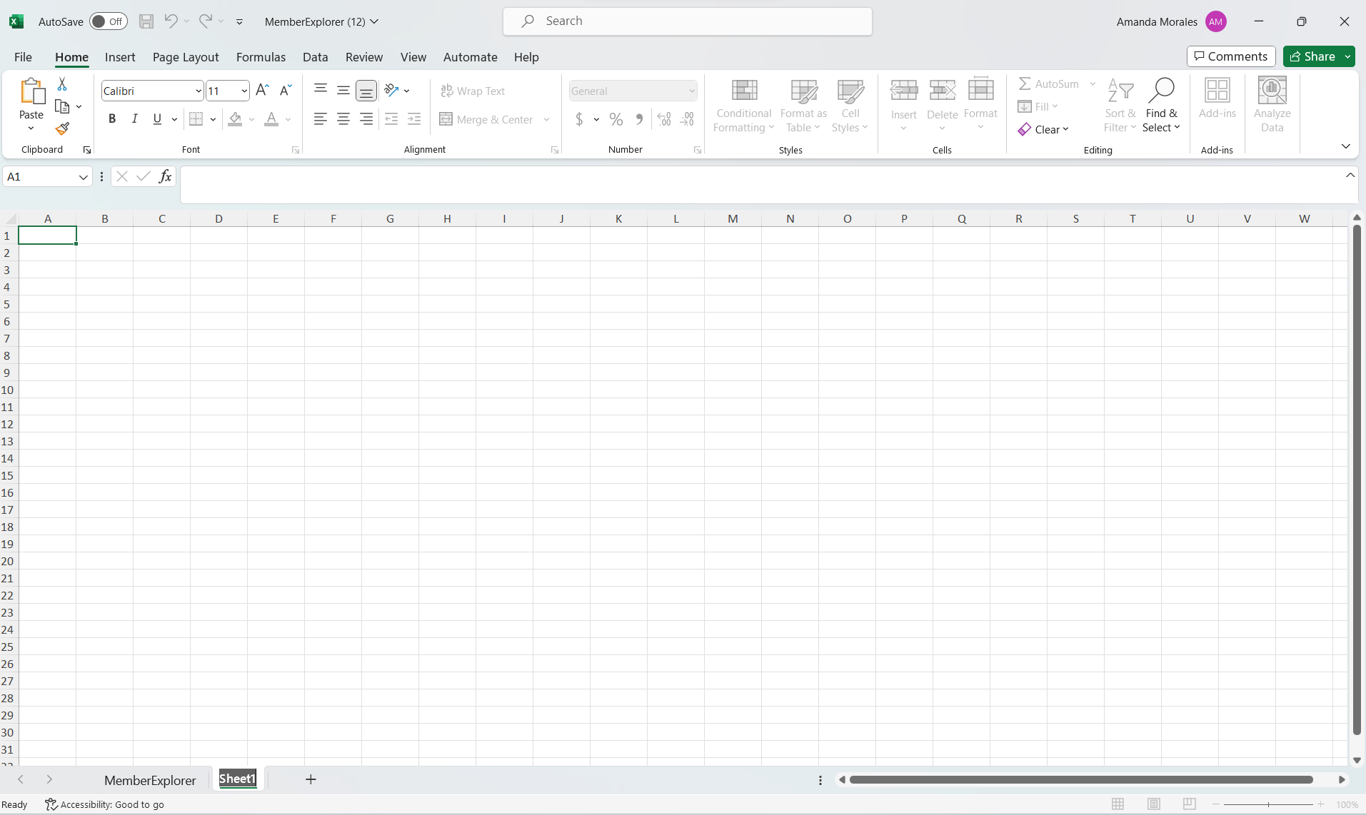
(2a) Open up the primary report (in this case the Member Explorer Download) and add a blank sheet in this same file. You can do this by clicking the small plus icon near the bottom of your screen.

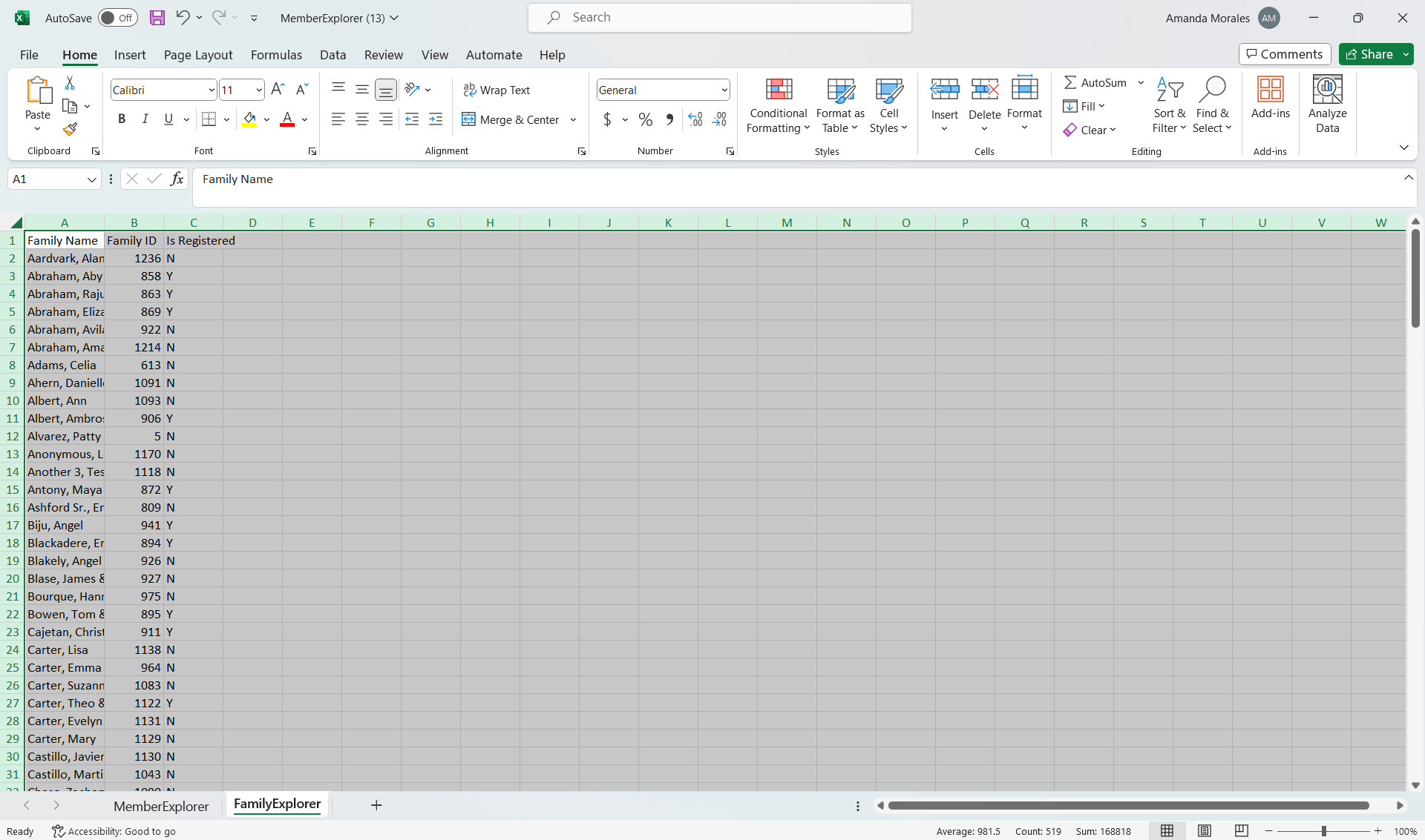
(2b) Copy all of the information from the secondary report (in our example, the Family Explorer download) and paste it in the blank tab of the primary download.
(2c) In the tab where your primary information is, add enough columns for the data you'd like to pull in from the secondary download. For instance, if I only want to pull the "Is Registered" field into the Member Explorer download, I'll need to add one column and list the header in row 1. If instead I were adding "Is Registered" and "Budget Number", I'd need to add 2 columns and list both headers in row 1.

Step 3: Entering the XLOOKUP formula for the first cell
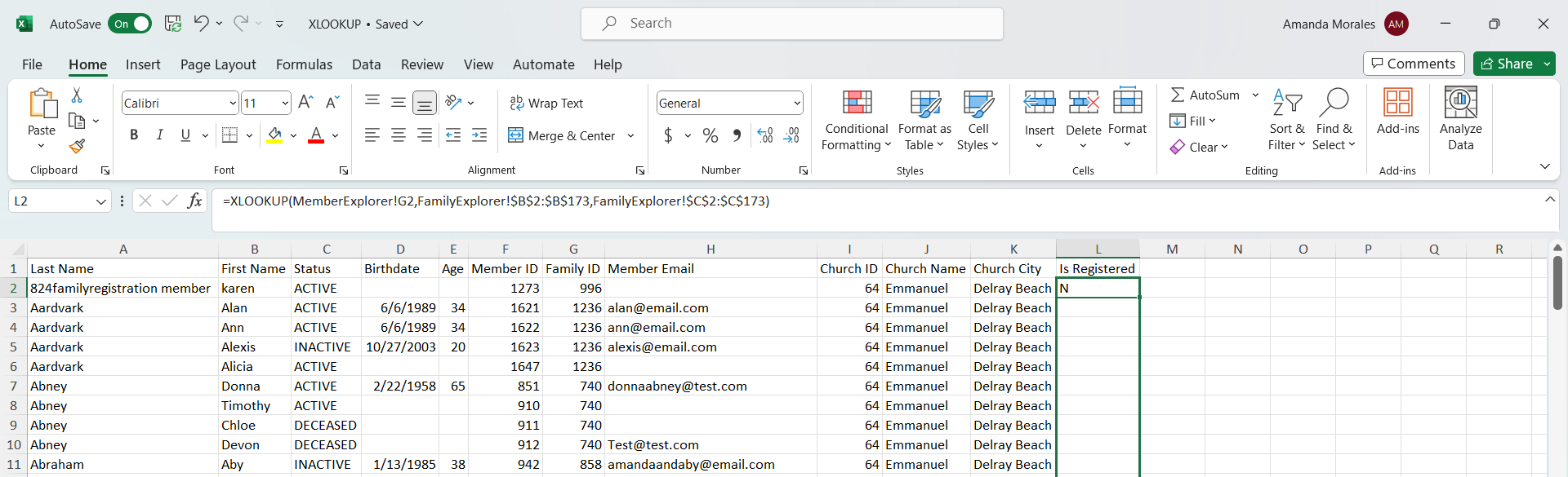
(3a) Now you will want to start by clicking into the first empty cell within the column you just added. In my example above, we will click into cell L2 (Column L, Row 2) which is the cell directly below where it says "Is Registered". You can see what cell you are clicked into by looking towards the top-left of your screen.

(3b) Begin typing =XLOOKUP(
Note: In Excel, the equal sign is what tells Excel you are going to begin typing a function/equation rather than typing text. XLOOKUP is the function we will be using. The open parentheses must be added before you can begin selecting the cells for your formula.
We will only be utilizing the required "arguments" which are the following:
- lookup_value - The cell Excel will search for.
- Our lookup_value will always be our most unique field which in most cases will be the Family ID, and it will be found on the primary download (Member Explorer). When Excel tells you "value" you know it wants a single cell. When it says "array" it's looking for a group of cells. Since we are typing this formula within cell L2, our corresponding lookup_value will be cell G2. We want to select G2 since it's within the same row as the cell we are clicked into, and it is under the Family ID column (Column G).
- lookup_array - The range of cells Excel will search within to find the lookup_value.
- Our lookup_array will be the range of cells that relates to our most unique field and is found on the secondary download. We will want to select the Family ID column within the secondary download. In this example you will see the range is B2:B173.
- return_array - The range of cells Excel will use to return the appropriate value when it locates the lookup_value within the lookup_array.
- Our return_array is the range of cells that will be used to return a single value when Excel locates the lookup_value within the lookup_array. In this example, my range should be C2:C173 which is the "Is Registered" column. (Sounds a little confusing? Stick with me! We'll get through this together 🙂)

Note: You will see "MemberExplorer!" and "FamilyExplorer!" within my formula. This is how Excel notes what tab you have selected the cell and/or range from. For instance, MemberExplorer!G2 means I've clicked on Cell G2 within my Member Explorer tab.
Important Note: Please note that specific cells and ranges are mentioned above (i.e. G2, B2:B173, and C2:C173). If you have more or less columns in your spreadsheet, your cells and ranges may differ. You will need to select the appropriate cells and ranges that make sense for your downloads.
Excel is going to search for the lookup_value within the lookup_array and when it finds it, it will gives us the corresponding value found in the return_array. In our specific example, Excel is searching for the first Family ID—Family ID 996 (cell G2)—within the "Family ID" column (B2:B173) found in the secondary tab. Once it locates Family ID 996, it will return the corresponding value found in the "Is Registered" column (C2:C173) of the secondary tab.
Step 4: Adding "Absolute Referencing"
(4) Absolute referencing allows you to "lock" the cell and/or range of cells you've selected. To add absolute referencing, you'll need to add a dollar sign to before the letter and number of the cell and/or range you've selected.
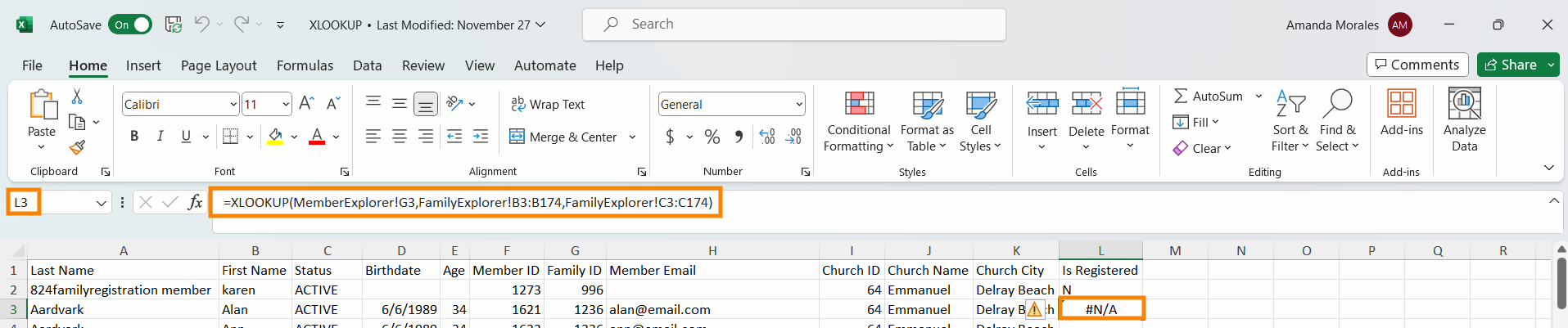
We want to do this because we will be "filling down" our formula, and in doing so Excel will change the formula slightly to reflect what it believes you're trying to accomplish. If I drag my formula down one row from L2 to L3, it will change the formula from =XLOOKUP(MemberExplorer!G2,FamilyExplorer!B2:B173,FamilyExplorer!C2:C173) to =XLOOKUP(MemberExplorer!G3,FamilyExplorer!B3:B174,FamilyExplorer!C3:C174). Notice how everything in the formula moved down one row. By doing this, we may not capture all of the data we have, because we are now excluding row 2.
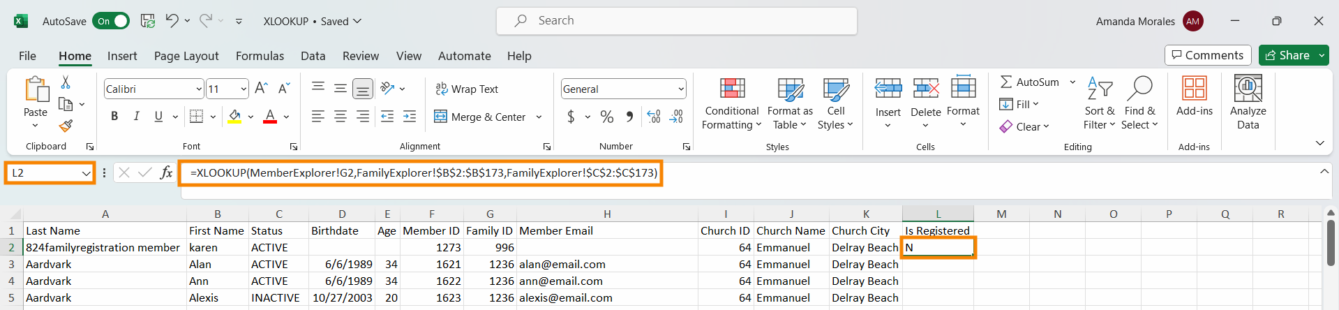
Click back into cell L2 and ensure you've added the dollar signs in the proper places. There should be a dollar sign before the letters and numbers within the lookup_array and return_array. Be sure not to add absolute referencing to the lookup_value. In our example, your formula in L2 should be: =XLOOKUP(MemberExplorer!G2,FamilyExplorer!$B$2:$B$173,FamilyExplorer!$C$2:$C$173)
Step 5: Fill down your formula
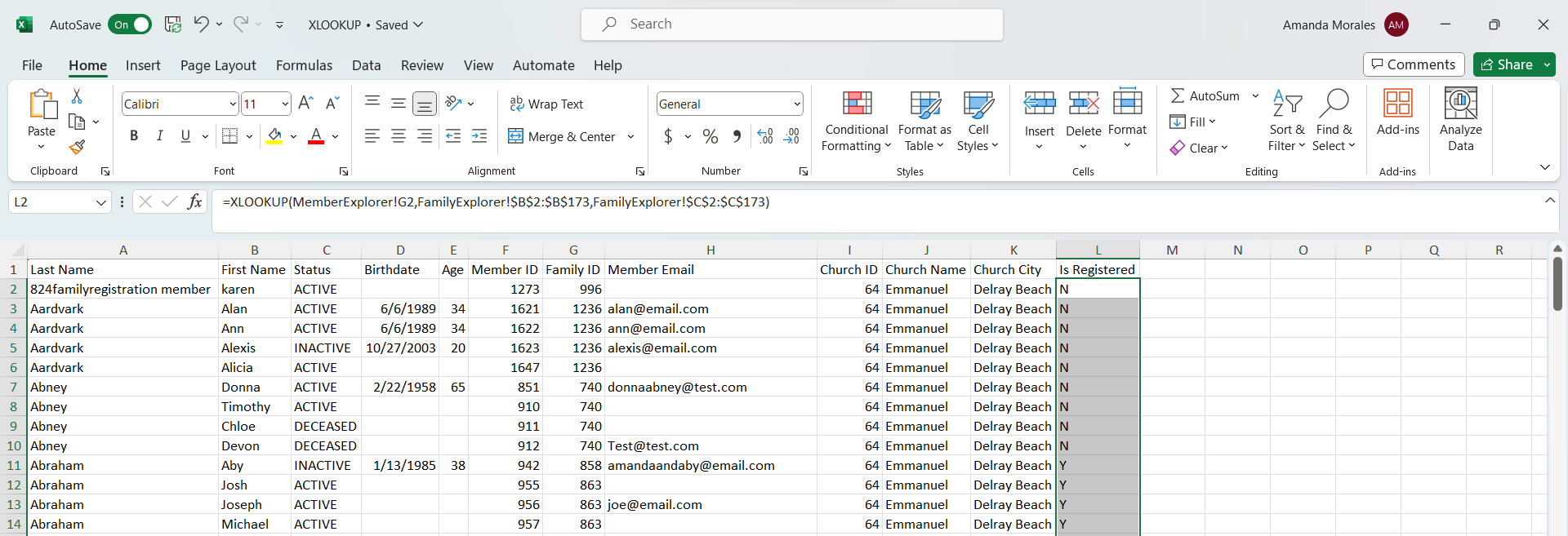
(5) We are now going to "fill down" our formula which will apply this (almost) same formula. I say almost because our lookup_value should change depending on which cell we are clicked into.
To fill down your formula, hover over the bottom-right corner of cell L2 or the cell where you first typed your formula in. You should see a little green box before you hover over the bottom-right corner, then you should see a small black plus icon.

Once you see this plus icon, click your mouse twice. You should then see your formula fill down. If you're having trouble with this, you can also drag the formula manually by waiting until you see the plus icon, click and hold your mouse as you drag until your last cell is selected.
Step 6 (optional): Tips and Tricks
(6a) You can apply this same logic to any other fields you want to add by adding more columns. Please see timestamp 23:02 in the video tutorial if you'd to see what this may look like.
(6b) You can turn your download into a table so you can easily sort and filter through your data. Perhaps you want to view Active members only, and only those members whose family is registered.
Step 7 (required): Celebrate!
(7) Great job! You did it! You should be proud of yourself for making it to the end of this article and successfully completing your XLOOKUP! 👏